Script to reproduce the paper
Nussbaumer, Raphaël, Grégoire Mariethoz, Mathieu Gravey, Erwan Gloaguen, and Klaus Holliger. 2017. “Accelerating Sequential Gaussian Simulation with a Constant Path.” Computers & Geosciences. Retrieved DOI:<http://linkinghub.elsevier.com/retrieve/pii/S0098300417304685 10.1016/j.cageo.2017.12.006>.
Contents
clc; addpath('..'); addpath('../functions');
Figure 1
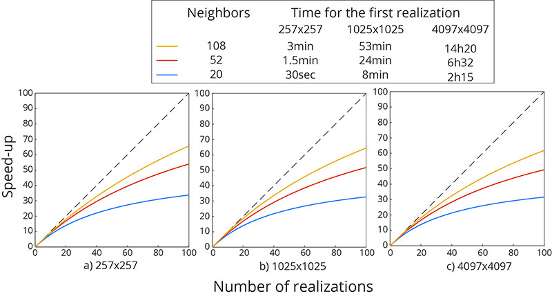
Speed-up as a function of the number of realizations performed for 3 differents grid sizes and neighbourhood sizes. The grid sizes were selected such that the multi-grid path is optimal and the neighbourhood size such that the resulting full neighbourhood is symmetric. The computational time for the first realization is also shown in the legend.
% General setting
covar.model = 'spherical';
covar.azimuth = 0;
covar.c0 = 1;
covar.alpha = 1;
covar.range0 = [15 15];

parm.seed_path = 'default';
parm.seed_search = 'shuffle';
parm.seed_U = 'default';
parm.saveit = 0;
parm.mg = 1;

neigh.wradius = 1;
m = 1;

% Define the range of grid size and neighborhood size
N=2.^[8 10 12]+1;%[257 1025 4097];
K=[20 52 108];

T_trad_g=nan(numel(N),numel(K));
T_cst_g=nan(numel(N),numel(K));
T_cst_real=nan(numel(N),numel(K));
T_trad_real =nan(numel(N),numel(K));

for i_n=1:numel(N)
    for i_k=1:numel(K)
        nx = N(i_n); % no multigrid
        ny = N(i_n);
        neigh.nb = K(i_k);

        [~,t] = SGS_cst(nx,ny,m,covar,neigh,parm);
        title = ['T_cst_' num2str(N(i_n)) 'N_' num2str(K(i_k)) 'K' ];
        T_cst_g(i_n,i_k) = t.global;
        T_cst_real(i_n,i_k) = t.real;

        [~,t] = SGS_trad(nx,ny,parm);
        title = ['T_trad_' num2str(N(i_n)) 'N_' num2str(K(i_k)) 'K' ];
        T_trad_g(i_n,i_k) = t.global;
        T_trad_real(i_n,i_k) = t.real;
    end
end

figure(1); clf
m=0:100;
for i_n=1:numel(N)
    subplot(1,numel(N),i_n); hold on
    plot([0 100],[0 100],'--k')
    for i_k=1:numel(K)
        eta = ( T_trad_g(i_n,i_k) + (m-1).*T_trad_real(i_n,i_k)) ./ ( T_cst_par_g(i_n,i_k) + (m-1).*T_cst_par_real(i_n,i_k));
        h(i_k)=plot(m,eta);
    end
    legend(h,{'20 Neighbors','52 Neighbors','108 Neighbors'});
    axis equal tight
    xlabel('Number of realizations')
    ylabel('Speed-up')
end
Reference to non-existent field 'range'.

Error in SGS_cst (line 44)
x = ceil( min(covar(1).range(2)*neigh.wradius, nx));

Error in script_paper (line 50)
        [~,t] = SGS_cst(nx,ny,m,covar,neigh,parm);
Figure 2,3,4
% General setting
covar.range0 = [15 15];
covar.azimuth = 0;
covar.c0 = 1;
covar.alpha = 1;

parm.seed_path = 'shuffle';
parm.seed_search = 'shuffle';
parm.saveit = 0;
parm.mg = 1;

neigh.wradius = 1;
neigh.nb = 20;

m = 1;
nx = 2^6+1;
ny = 2^6+1;

% Defines the type of variogram tested
vario = {'exponential', 'gaussian', 'spherical', 'hyperbolic','k-bessel', 'cardinal sine'};

% Compute the true covariance fo each covariance model
[Y, X] = ndgrid(1:nx,1:ny); XY = [Y(:) X(:)];
for v=1:numel(vario)
    covar.model = vario{v};
    covar = kriginginitiaite(covar);
    DIST = squareform(pdist(XY*covar.cx));
    CY_true{v} = kron(covar.g(DIST), covar.c0);
end
err_frob_fx = @(CY,v) sqrt(sum((CY(:)-CY_true{v}(:)).^2)) / sum((CY_true{v}(:).^2));


% Simulation
N = 10;
vario_g=cell(numel(vario),1);
D = pdist2(XY,XY);
h = unique(D);
h = h(h<=parm.k.covar.range0(1)*1.5);

parfor v=1:numel(vario)
    parm1=parm;
    parm1.gen.covar.model = vario{v};
    CY=repmat({nan(ny*nx,nx*ny,2)},N,1);
    eta{v}=cell(N,1);
    nn=cell(N,1);
    for n=1:(2^(N-1))
        vec = de2bi(n-1,N);
        CY{1}(:,:,vec(1)+1) = full(SGS_varcovar(nx,ny,parm1));
        eta{v}{1} = [eta{v}{1}; err_frob_fx(CY{1}(:,:,vec(1)+1),v)];
        nn{1} = [nn{1}; 2^(1-1)];
        i=1;
        while (vec(i)==1)
            CY{i+1}(:,:,vec(i+1)+1) = mean(CY{i},3);
            eta{v}{i+1} = [eta{v}{i+1}; err_frob_fx(CY{i+1}(:,:,vec(i+1)+1),v)];
            nn{i+1} = [nn{i+1}; 2^(i)];
            i=i+1;
        end
        disp(['N: ' num2str(n) ])
    end

    vario_g{v} = nan(N,numel(h));
    for n=1:N
        for i=1:numel(h)
            id = D ==h(i);
            id2 = CY{n}(id);
            vario_g{v}(n,i) = sum(id2)/sum(id(:));
        end
    end
end

% Save result
%save(['./cst_path_paper/frobenium_65n_20k_512N_1MG'],'eta','vario','vario_g','n','parm','nx','ny');
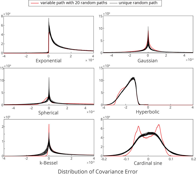
Figure 2
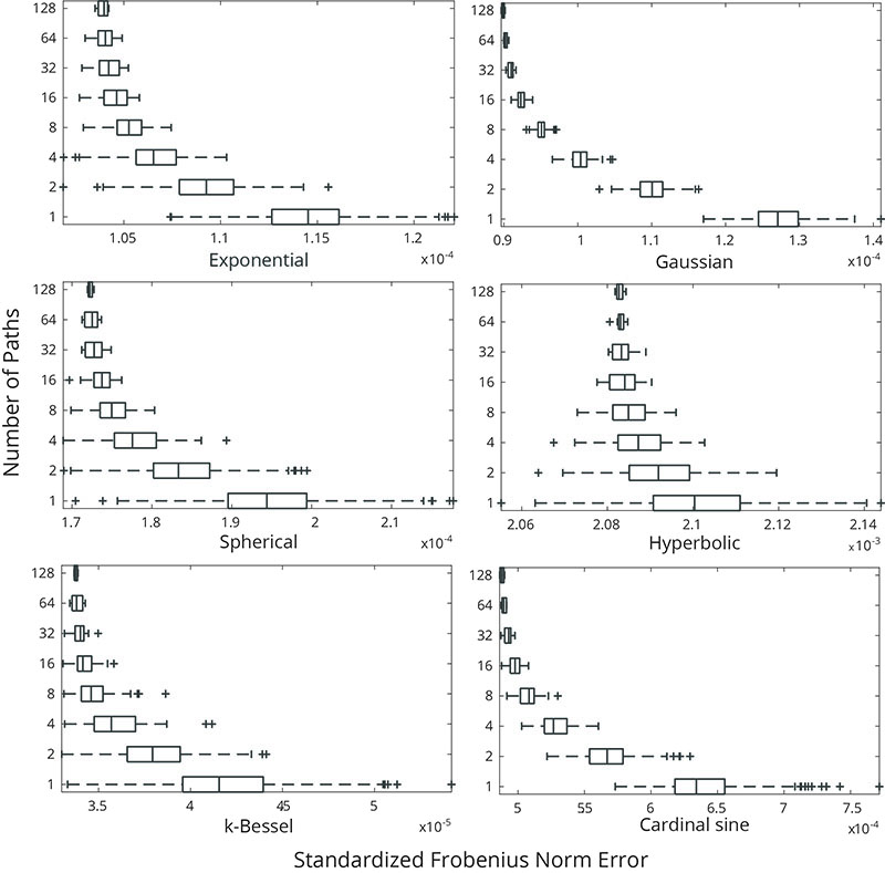
Boxplots of the SFN of simulated RFs  for different numbers of simulation paths
  . 512 simulated RFs
  were computed and different numbers of them combined to construct the simulated RFs with a fully randomized path according to equation 20.
figure(2);clf; hold on;
lim=8;
load('Y:/SGS/cst_path_paper/frobenium_65n_20k_512N_1MG');
for v=1:numel(vario)
    subplot(numel(vario)/2,2,v); hold on;
    boxplot(cell2mat(eta{v}(1:lim)),cell2mat(nn(1:lim)),'Orientation','horizontal','Color',[0 113 188]/255);
    axis tight;
    xlabel(['Number of Path\newline' vario{v} ' variogram']);
    ylabel(['Standardized Frobenius Norm Error'])
end
Figure 3
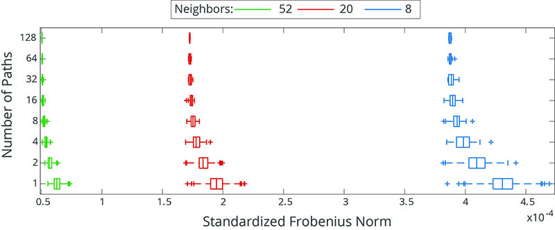
Boxplot of the SFN for several simulated RFs for different numbers of simulation paths and different neighbourhood sizes for a spherical covariance function.
figure(3); clf; hold on;
lim=8;
filename2={'frobenium_sph_8_512', 'frobenium_sph_20_512' ,'frobenium_sph_52_512'};
col={'b','r','g','y'};
for i=1:numel(filename2)
    s=load(['result-SGSIM/Constant Path/' filename2{i}]);
    xlim_b=get(gca,'xlim');
    boxplot(cell2mat(s.eta(1:lim)),cell2mat(nn(1:lim)),'Orientation','horizontal','color',col{i},'symbol',['+' col{i}]);
    xlim_a=get(gca,'xlim');
    if i>1
        xlim([ min(xlim_b(1), xlim_a(1)) max(xlim_b(2), xlim_a(2))])
    end
end
hLegend = legend(findall(gca,'Tag','Box'), {'Neighboors: 8', 'Neighboors: 20', 'Neighboors: 52'});
ylabel('Number of Path');
xlabel('Standardized Frobenius Norm Error')
Figure 4
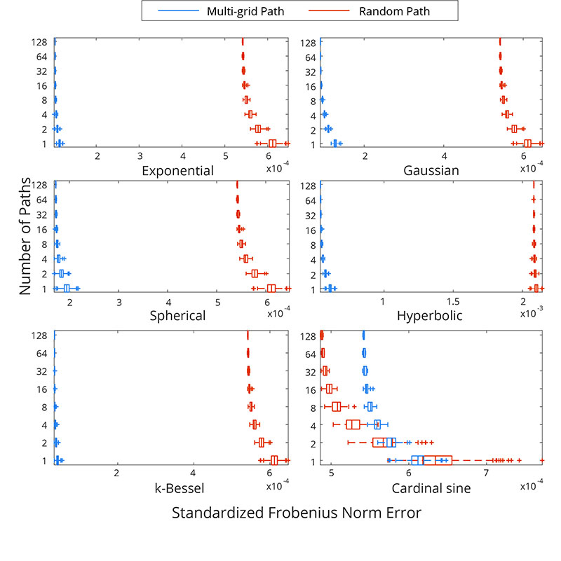
Boxplot of the SFN for several simulated RFs using different numbers of simulation paths for multi-grid or random simulation paths.
figure(4);clf;
lim=8;
filename2={'frobenium_65n_20k_512N_0MG' ,'frobenium_65n_20k_512N_1MG'};
col={'b','r','g','y'};
for v=1:numel(vario)
    subplot(numel(vario)/2,2,v); hold on;
    for i=1:numel(filename2)
        s=load(['Y:/SGS/cst_path_paper/' filename2{i}]);
        xlim_b=get(gca,'xlim');
        boxplot(cell2mat(s.eta{v}(1:lim)),cell2mat(nn(1:lim)),'Orientation','horizontal','color',col{i},'symbol',['+' col{i}]);
        xlim_a=get(gca,'xlim');
        if i>1
            xlim([ min(xlim_b(1), xlim_a(1)) max(xlim_b(2), xlim_a(2))])
        end
    end
    hLegend = legend(findall(gca,'Tag','Box'), {'Random Path', 'Mutli-grid Path'});
    ylabel('Number of Path');
    xlabel('Standardized Frobenius Norm Error')
end
Figure 5
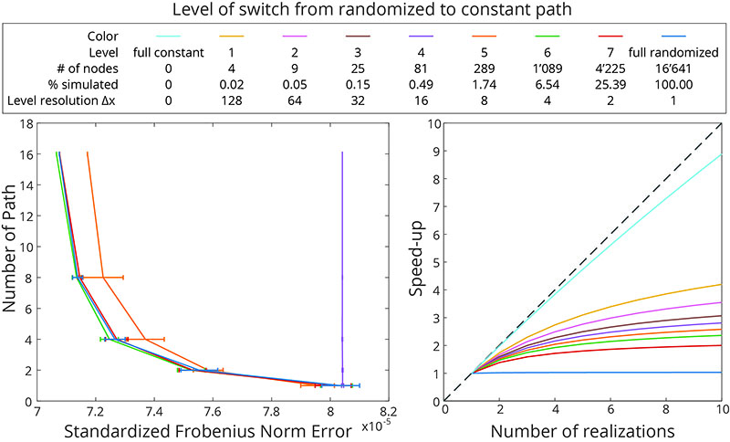
(Left) Mean and standard deviation of the SFN using up to 16 different randomized multi-grid paths for simulations where the constant path approach is switched on at different grid level. Note that the curves for levels 1-4 and for the fully constant path are superimposed. (Right) Corresponding simulation speed-up of simulation.
% General setting
covar.model = 'gaussian';
covar.range0 = [15 15];
covar.azimuth = 0;
covar.c0 = 1;
covar.alpha = 1;

parm.seed_path = 'shuffle';
parm.seed_search = 'shuffle';
parm.saveit = 0;
parm.mg = 1;

neigh.wradius = 1;
neigh.nb = 20;

m = 1;
nx = 2^7+1;
ny = 2^7+1;

% Build true covariance matrice
[Y, X]=ndgrid(1:nx,1:ny); XY = [Y(:) X(:)];
covar = kriginginitiaite(parm.k.covar);
DIST = squareform(pdist(XY*covar.cx));
CY_true = kron(covar.g(DIST), covar.c0);
err_frob_fx = @(CY) sqrt(sum((CY(:)-CY_true(:)).^2)) / sum((CY_true(:).^2));

N=2;
CY=repmat({nan(ny*nx,nx*ny,2)},N,1);
eta=cell(N,1);
nn=cell(N,1);
for n=1:(2^(N-1))
    vec = de2bi(n-1,N);
    CY{1}(:,:,vec(1)+1) = full(SGS_varcovar(nx,ny,parm));
    eta{1} = [eta{1}; err_frob_fx(CY{1}(:,:,vec(1)+1))];
    nn{1} = [nn{1}; 2^(1-1)];
    i=1;
    while (vec(i)==1)
        CY{i+1}(:,:,vec(i+1)+1) = mean(CY{i},3);
        eta{i+1} = [eta{i+1}; err_frob_fx(CY{i+1}(:,:,vec(i+1)+1))];
        nn{i+1} = [nn{i+1}; 2^(i)];
        i=i+1;
    end
    disp(['N: ' num2str(n) ])
end

sx = 1:ceil(log(nx+1)/log(2));   sy = 1:ceil(log(ny+1)/log(2));   sn = max([numel(sy), numel(sx)]);
nb = nan(sn,1);start = zeros(sn+1,1);   path = nan(nx*ny,1); Path = nan(ny,nx);
for i_scale = 1:sn
   dx(i_scale) = 2^(sn-sx(min(i_scale,end))); dy = 2^(sn-sy(min(i_scale,end)));
   [Y_s,X_s] = ndgrid(1:dy:ny,1:dx(i_scale):nx); % matrix coordinate
   id = find(isnan(Path(:)) & ismember(XY, [Y_s(:) X_s(:)], 'rows'));
   nb(i_scale) = numel(id); start(i_scale+1) = start(i_scale)+nb(i_scale);
   path( start(i_scale)+(1:nb(i_scale)) ) = id(randperm(nb(i_scale)));
   Path(path( start(i_scale)+(1:nb(i_scale)) )) = start(i_scale)+(1:nb(i_scale));
end

% save(['./cst_path_paper/frobenium_129n_20k_16N_MG_' num2str(parm.seed_path) 'CSTP'],'eta','nn','parm','nx','ny','nb');


% Figure
figure(10);clf; hold on;
CST=1:9; cnb = cumsum(nb); ldgd=cell(numel(CST),1);
for i = 1:numel(CST)
    load(['Y:/SGS/cst_path_paper/frobenium_129n_20k_16N_MG_' num2str(CST(i)) 'CSTP'])
    %boxplot(cell2mat(eta),cell2mat(nn),'Orientation','horizontal','Color',[0 113 188]/255);
    M = cellfun(@median,eta);
    S = cellfun(@std,eta);
    n = flipud(cellfun(@numel,eta));
    errorbar(n,M,S)
    ldgd{i} = ['Level ' num2str(CST(i)-1) ' (' num2str(cnb(CST(i)-1)) ' nodes | ' num2str(cnb(CST(i)-1)./cnb(end)*100,'%4.2f') '% | \Deltax=' num2str(dx(CST(i)-1)) ')' ];
end
view(90,-90); box on
xlabel('Number of Path');
ylabel('Standardized Frobenius Norm Error')
title('Constant path from level x with Multi-grid');

legend(ldgd)


% General setting
parm.k.covar.model = 'spherical';
parm.k.covar.azimuth = 0;
parm.k.covar.c0 = 1;
parm.k.covar.alpha = 1;
parm.seed_search = 'shuffle';
parm.k.covar.range0 = [15 15];
parm.k.wradius = 3;
parm.mg = 1;
nx = 2^7+1; % no multigrid
ny = 2^7+1;
parm.k.nb = 20;

seed_path=1:9;

nt=2;
t_real=nan(nt,numel(seed_path));
t_global=nan(nt,numel(seed_path));
for j=1:numel(seed_path)
    parm.seed_path = seed_path(j);
    for i=1:nt
        profile on
        [~,t] = SGS_hybrid(ny,nx,parm);
        profile viewer
        t_global(i,j)=t.global-t.covtable;
        t_real(i,j)=t.real;
    end
end


clear eta;
m=1:10;
for i_m=m
    eta(i_m,:) = i_m.*mean(t_global) ./ ( mean(t_global) + (i_m-1).*mean(t_real));
end

figure(5); clf; hold on;
plot(eta)
plot([0 10], [0 10], '--k')
legend(ldgd);
axis tight equal
xlabel('Number of realizations')
ylabel('Speed-up')
Figure 6
Older version of the code not maintained...